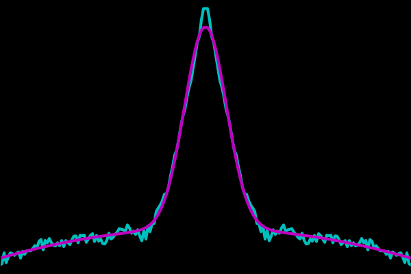
A colleague recently asked for help getting the functionality of IDL’s GAUSSFIT function working in Python. This was a perfect opportunity to use the handy curve_fit function from SciPy. Here’s the code:

import numpy as np
from scipy.optimize import curve_fit

xdata, ydata = np.loadtxt('focus_output.dat', unpack=True)

def fit_func(x, a0, a1, a2, a3, a4, a5):
    z = (x - a1) / a2
    y = a0 * np.exp(-z**2 / a2) + a3 + a4 * x + a5 * x**2
    return y

parameters, covariance = curve_fit(fit_func, xdata, ydata)

The file focus_output.dat just contains some data in two columns of numbers. For more info on loadtxt see my post on reading text tables. fit_func defines the function we want to fit to the data. In this case it is a Gaussian plus a quadratic, the same as used in GAUSSFIT when NTERMS=6. Now, to plot the results:

import matplotlib.pyplot as plt

fitdata = fit_func(xdata, *parameters)

fig = plt.figure(figsize=(6,4), frameon=False)
ax = fig.add_axes([0, 0, 1, 1], axisbg='k')

ax.plot(xdata, ydata, 'c-', xdata, fitdata, 'm-', linewidth=3)

ax.set_ylim(0.38, 1.02)

fig.savefig('gauss_fit_demo.png')