IPython Notebook Viewer

The nice folks over at IPython have put together a nice viewer for IPython notebooks stored as GitHub gists: nbviewer.ipython.org/. Just enter a gist URL or number. It doesn’t actually store notebooks, just renders notebooks stored as gists.

I’ve had some notebooks as gists for a while and now I can make pretty links to them:

IPython Notebook Viewer

Upgrading to Mountain Lion

I just upgraded to Mountain Lion and here are some of my notes related to scientific Python installs.

If you’ve already got a working installation it will likely continue to work after upgrading. Regardless of whether you plan to keep using an existing install or make a new one you’ll probably want to do the following two things:

Xcode

You’ll need a Mountain Lion compatible set of command line tools and development libraries so reinstall Xcode or the Command Line Tools for Xcode. I personally prefer the later now that I use Sublime Text 2 for code editing. If you install Xcode make sure to install the command line tools from the preferences.

X11

ML doesn’t come with X11 installed so install XQuartz from http://xquartz.macosforge.org/ if you anticipate needing X11.

Python Libraries

  • NumPy compiles without issue.
  • SciPy is waiting on a small change before it will compile on Mountain Lion. I expect that to go in soon and they may release SciPy 0.10.2 to make it Mountain Lion compatible. Even if they don’t you’ll be able to install from the GitHub repository once the change is made.
  • matplotlib must be installed from the GitHub repository at this time.
Upgrading to Mountain Lion

brewer2mpl – colorbrewer2 and Python

A friend recently tweeted: “Who knows of a python code that intelligently picks colors based on the number needed for a plot?” Phil is plotting several datasets on one plot and wanted an easy way to get a good set of colors to use. I mentioned colorbrewer2.org, which has terrific color maps, but they are locked up in a Flash application. So I had the idea to make a Python package bringing the colorbrewer2.org color maps into Python and connecting them to matplotlib.

There is an existing Python package called colorbrewer but it’s undocumented, doesn’t have its code in a public repository, and is missing some features I wanted. (And it was updated for the first time in 3 years on the day I wrote this post.) It also turns out that the colorbrewer2.org color maps are already in matplotlib (all the capitalized maps in this example) but that doesn’t give access the original colors as defined by colorbrewer2.org. And so was born brewer2mpl.

colorbrewer2.org has three types of color maps: sequential, diverging, and qualitative (for categorical data). Each color map is defined several times with different numbers of colors, anywhere from three to 12.

brewer2mpl packages the colorbrewer2.org color maps and gives access to them as 0-255 RGB triplets, 0-1 RGB triplets, hex strings, and matplotlib color maps. It contains functions for listing color maps by type and number of defined colors. Now Phil can do the following to get some good colors to use in matplotlib plots:

import brewer2mpl
bmap = brewer2mpl.get_map('Set1', 'qualitative', 5)
colors = bmap.mpl_colors

For more information:

This was my first time building and releasing my own package. It was fun and a great chance to learn about the simplest aspects of releasing Python packages. (Nothing fancy going on here.) Hope I get the chance to do more!

brewer2mpl – colorbrewer2 and Python

SciPy 2012

Last week was the SciPy 2012 conference in Austin, TX. I’ve been for the last three years and it’s a good event for the tutorials on scientific Python packages, to see what crazy fields people are using Python in (brain-robotics interaction!), to hack on your favorite project, and to meet the maintainers of some of the packages you use every day. I recommend it especially to people who are new to scientific Python as you’ll learn a lot your first year. All of the tutorials and talks from SciPy are recorded and should be up on the web soon. You can also check out the #scipy2012 stream on Twitter.

Tutorials

This year I went to tutorials on scikits-learn, HDF5 with PyTables, pandas, and IPython:

scikits-learn

scikits-learn is the package for machine learning in Python. I haven’t had occasion to use it but if I ever need to do ML scikits-learn will be the first tool I reach for. The documentation is excellent and the interfaces seem simple and logical. Jake VanderPlas’ excellent tutorial is online at http://astroml.github.com/sklearn_tutorial/.

HDF5 with Pytables

HDF5 is a data format that can handle pretty much any kind of data, and when paired with PyTables it seems to be especially useful for efficiently working with very large datasets. One nice feature of HDF is that you can put many different arbitrary datasets in one file and attach separate metadata to every node of the file.

pandas

pandas has been skyrocketing in popularity lately and for good reason. If you’re working with time series or tabular data pandas is probably the tool you should be using. pandas has extremely slick indexing and slicing, handling of missing data, and intelligent data alignment. The DataFrame object supports SQL-like merging and joining. Time handling is really amazing. pandas supports time zones and daylight saving time. It has really rich support for different periods and frequencies. If you’re working with time series or tabular data you should really give pandas a try.

Ipython

I’ve written about IPython before. The notebook is the big star these days and they demoed some really cool features, including making interactive plots with JavaScript. All of their tutorial notebooks are available on GitHub and I recommend you check them out if you’re curious about all the crazy stuff the notebook can do.

Talks

All of the talks are listed on the SciPy website. Many of the talks tend to be very domain specific but the keynotes are always interesting. This year John  Hunter talked about the growth of matplotlib and Joshua Bloom talked about how he has used Python throughout his astronomy career, from machine learning to remotely controlling telescopes.

The theme of SciPy 2012 seemed to be high powered computing. This has been the case in years past, but while in previous years the focus has been on the cloud or GPUs, this year seemed to be about serial optimization using fancy compilers, especially LLVM. Numba and Julia seemed to be stars of the conference in this respect. (Julia isn’t actually related to Python, but the language syntax does look a lot like Python. People seemed especially excited about the prospect of calling Julia from Python much as you can call C from Python. Anything to not have to work in C…)

One thing that caught my eye during the lightning talks was pipe-o-matic, a Python tool for making data pipelines. It’s still coming together but I could see it being useful. Pipelines are defined in simple text files and the executables and their versions are fully specified. This means you can archive/version control your pipelines along with your data to track which versions of which programs were used to make the data. pipe-o-matic supposedly has full support for resuming or restarting pipelines after errors. It looks simple and lightweight.

Astronomy Mini-Symposium

This year there were topical mini-symposia on geophysics, astronomy, meteorology, and bioinformatics. The astronomy talks included AstroPy, astroML for machine learning in astronomy, and the yt visualization toolkit for astronomical simulations. yt makes some seriously beautiful visualizations.

It was great to have the topical symposium and see what others are doing with Python in astronomy, I hope these sessions keep showing up at SciPy and other places. Maybe AAS should have some Python sessions?

Sprints

This was my first year participating in the sprints, which are basically hack days where project developers will organize groups of programmers to tackle certain issues in their projects. There were groups working on scikits-learn, scikits-image, AstroPy, matplotlib, IPython and more. I ended up working on my own project, brewer2mpl, which I will discuss in another blog post.

Other Thoughts

Each time I’ve been to SciPy over the last three years I’ve been struck by how few women are there (~2% of attendees). Maybe I shouldn’t be shocked to see so few women at a conference on scientific programming, but it’s really pathetic, and it would be nice to see the organizers make an effort to recruit a more diverse group of attendees. I think a significant fraction of the women at SciPy 2012 were astronomers, keep up the good work astronomy!
SciPy 2012

Profiling Python

Profiling a program is a way to take a detailed look at the execution time of individual pieces of the program. When you want to optimize code it’s important to use a profiler first so that you know where your optimization effort would be most beneficial.

I recently demonstrated profiling Python code using the built-in tools, line_profiler, and IPython’s “magic” hooks into those tools. RunSnakeRun also made an appearance.

As usual I used the IPython notebook and you can get the .ipynb file and the PDF, or see it directly.

More info on using the built-in profiler and pstats modules is available via the Python Module of the Week: http://www.doughellmann.com/PyMOTW/profile/index.html.

Profiling Python

pandas in the IPython Notebook

I finally got around to playing a tiny bit with pandas today and was delighted when I saw its representation in the IPython notebook. Take a look in the PDF.

IPython detects a special _repr_html_ method on (in this case) the pandas DataFrame object and uses that for the output instead of the usual __str__ or __repr__ methods. Here _repr_html_ returns the contents of the DataFrame in an HTML table, which is also useful for posting to a blog:

Ant Bat Cat Dog
0 0 1 2 3
1 4 5 6 7
2 8 9 10 11
3 12 13 14 15
4 16 17 18 19

This is another great feature of the IPython notebook and I look forward to it popping up in more places!

pandas in the IPython Notebook

Fuzzy Floating Point Comparison

I was writing some tests today and I ran into a peculiar floating point issue. I had generated a sequence of numbers using numpy.linspace:

>>> np.linspace(0.1, 1, 10) 
array([ 0.1, 0.2, 0.3, 0.4, 0.5, 0.6, 0.7, 0.8, 0.9, 1. ])

Part of the code I was testing ended up testing whether the value 0.3 was in the range 0.3 – 0.8, including the end points. The answer should of course be yes, but there is a twist due to the actual values in the array returned by linspace:

>>> a = np.linspace(0.1, 1, 10)
>>> 0.3 in a
False
>>> 0.3 < a[2]
True

What’s happening is that the 0.3 returned by linspace is really 0.30000000000000004, but the 0.3 when I type 0.3 is really 0.29999999999999999. It’s not clear whether this situation would ever actually arise in the normal usage of the code I was testing, but I wanted to make sure this wouldn’t cause problems. My solution was to make a function which would test whether a value was in a given range with a tiny bit of fuzziness at the edges.

NumPy has a useful function for comparing floating point values within tolerances called allclose. But that’s for comparing equality, I need fuzzy (but not very fuzzy) less than / greater than comparisons. To provide just that little bit of fuzziness I turned to the numpy.nextafter function.

nextafter gives the next representable floating point number after the first  input value. The second input value controls the direction so you can get the next value either up or down. It turns out that the two numbers that are tripping me up are right next to each other in their floating point representation:

>>> np.nextafter(0.29999999999999999, 1)
0.30000000000000004
>>> np.nextafter(0.30000000000000004, 0)
0.29999999999999999

So to catch this case my range checking function only needs one ULP of fuzziness (which is not much at all) to handle this floating point error. To allow for this I wrote a function called fuzzy_between that takes a value and the lower and upper bounds of the test range and expands the test range by a couple ULP before doing a simple minval <= val <= maxval comparison:


import numpy as np

def fuzzy_between(val, minval, maxval, fuzz=2, inclusive=True):
    """
    Test whether a value is within some range with some fuzziness at the edges
    to allow for floating point noise.

    The fuzziness is implemented by expanding the range at each end `fuzz` steps
    using the numpy.nextafter function. For example, with the inputs
    minval = 1, maxval = 2, and fuzz = 2; the range would be expanded to
    minval = 0.99999999999999978 and maxval = 2.0000000000000009 before doing
    comparisons.

    Parameters
    ----------
    val : float
        Value being tested.

    minval : float
        Lower bound of range. Must be lower than `maxval`.

    maxval : float
        Upper bound of range. Must be higher than `minval`.

    fuzz : int, optional
        Number of times to expand bounds using numpy.nextafter.

    inclusive : bool, optional
        Set whether endpoints are within the range.

    Returns
    -------
    is_between : bool
        True if `val` is between `minval` and `maxval`, False otherwise.

    """
    # expand bounds
    for _ in xrange(fuzz):
        minval = np.nextafter(minval, minval - 1e6)
        maxval = np.nextafter(maxval, maxval + 1e6)

    if inclusive:
        return minval <= val <= maxval

    else:
        return minval < val < maxval

For a great discussion on comparing floating point numbers see this randomascii post, and for some interesting discussion on the fallibility of range functions see this post on Google+ by Guido van Rossum. Guido actually calls out numpy.linspace as a range function not susceptible to floating point drift (since it’s calculating intervals, not adding numbers), but it’s always possible to get surprises with floating point numbers.

Fuzzy Floating Point Comparison

Python imhead and hedit

Working at STSCI I frequently deal with FITS files and while working on the new CALACS pipeline I often needed to see and change header values to run CALACS under different regimes. This can be done with IRAF tasks imhead and hedit but I try to use IRAF as little as possible.

PyFITS has convenience functions for working with FITS headers but as of version 3.0.7 it doesn’t come with any scripts that make them accessible from the command line. I expect that soon PyFITS and/or AstroPy will have these scripts, but in the meantime here are the ones I use. Continue reading “Python imhead and hedit”

Python imhead and hedit

IPython HTML Notebook

Until recently I had never been a fan of IPython but with their HTML notebook they’ve finally won me over. What I like about this tool is that it makes it easy to go back and forth between interactive prototyping and a script. Being able to continuously edit and re-run code in an interactive session is a powerful tool.

The notebook also makes a great tutorial and demo tool. Here’s a PDF of my session developing a Python replacement for IDL’s GAUSSFIT function.

Installation

The IPython notebook requires a few extra packages but if you have a setup like me it’s easy to get everything installed:

brew install zeromq
pip install pyzmq
pip install tornado
pip install ipython

After doing this you may also want to locally install MathJax for JavaScript equation rendering:

from IPython.external.mathjax import install_mathjax
install_mathjax()

To launch the notebook from whatever directory you want to work in:

ipython notebook

This will launch the IPython notebook dashboard in your default browser, from which you can make new notebooks or resume working on existing ones.

See the docs for all you can do with the notebook, and enjoy!

IPython HTML Notebook

IDL’s GAUSSFIT in Python

A colleague recently asked for help getting the functionality of IDL’s GAUSSFIT function working in Python. This was a perfect opportunity to use the handy curve_fit function from SciPy. Here’s the code:

import numpy as np
from scipy.optimize import curve_fit

xdata, ydata = np.loadtxt('focus_output.dat', unpack=True)

def fit_func(x, a0, a1, a2, a3, a4, a5):
    z = (x - a1) / a2
    y = a0 * np.exp(-z**2 / a2) + a3 + a4 * x + a5 * x**2
    return y

parameters, covariance = curve_fit(fit_func, xdata, ydata)

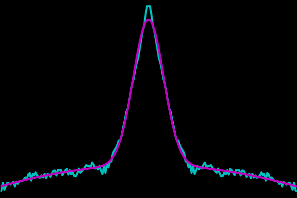
The file focus_output.dat just contains some data in two columns of numbers. For more info on loadtxt see my post on reading text tables. fit_func defines the function we want to fit to the data. In this case it is a Gaussian plus a quadratic, the same as used in GAUSSFIT when NTERMS=6. Now, to plot the results:

import matplotlib.pyplot as plt

fitdata = fit_func(xdata, *parameters)

fig = plt.figure(figsize=(6,4), frameon=False)
ax = fig.add_axes([0, 0, 1, 1], axisbg='k')

ax.plot(xdata, ydata, 'c-', xdata, fitdata, 'm-', linewidth=3)

ax.set_ylim(0.38, 1.02)

fig.savefig('gauss_fit_demo.png')

Data and Fitted Function
Cyan shows the original data, magenta shows the function fit with parameters returned by curve_fit.
IDL’s GAUSSFIT in Python